Causal Modeling &
Mediation Analysis

Data-based Storytelling

Daniel Winkler

Institute for Retailing & Data Science

Nils Wlömert

Types of analyses

• Descriptive - What has happened?
• Predictive - What will happen?
• Causal - Why does it happen?
• Prescriptive - What actions should be taken?

Descriptive

library(readr)
library(stringr)
library(tidyverse)
library(data.table)
library(scales)
time_series_ggstyle <- list(
  scale_y_continuous(labels = label_number(scale_cut = cut_si(' ')), expand = c(0, 0.1)),
  theme_bw(base_size = 20),
  theme(
    axis.title.x = element_blank(),
    panel.border = element_blank(),
    axis.line = element_line(color = "black"),
    legend.position = 'top'
  )
)
options(scipen = 99999)
charts <- fread("data/charts_at_global.csv.gz")
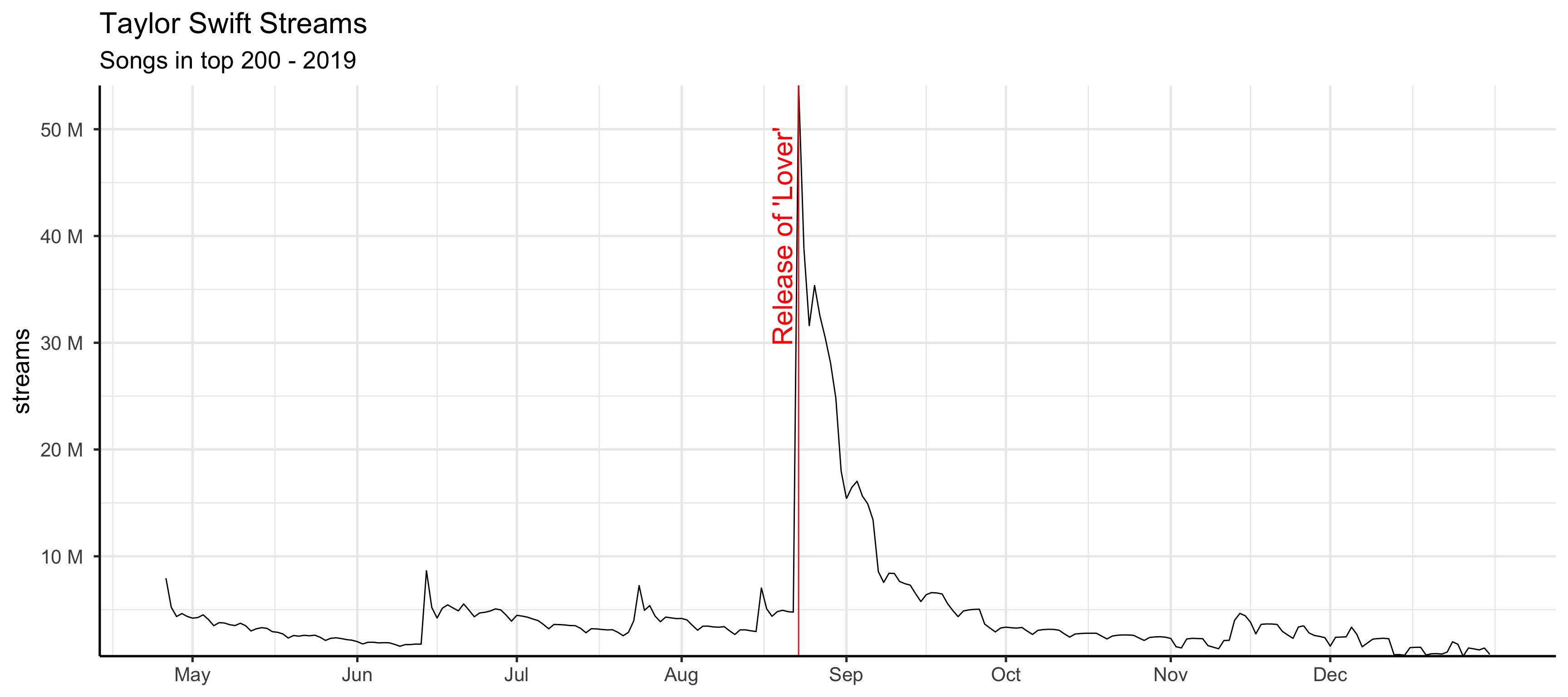
ts <- str_detect(tolower(charts$artistName), "taylor swift")
charts_ts <- charts[ts, ]
filter(charts_ts, format(day, "%Y") == "2019" & region == "global") |>
  group_by(day) |>
  mutate(streams = sum(streams)) |>
  ggplot(aes(x = day, y = streams)) +
  geom_line() +
  scale_x_date(
    breaks = seq(as.Date("2019-01-01"), as.Date("2019-12-31"), "month"),
    date_labels = "%b"
  ) +
  geom_vline(xintercept = as.Date("2019-08-23"), color = "red") +
  annotate("text", x = as.Date("2019-08-20"), label = "Release of 'Lover'", y = 40000000, colour = "red", angle = 90, size = 8) +
  ggtitle("Taylor Swift Streams", subtitle = "Songs in top 200 - 2019") +
  time_series_ggstyle

Predictive

library(zoo)
library(prophet)
total_streams <- charts |>
  filter(region == "global") |>
  group_by(day) |>
  summarize(y = sum(streams)) |>
  mutate(ds = as.Date(day)) |>
  select(-day)
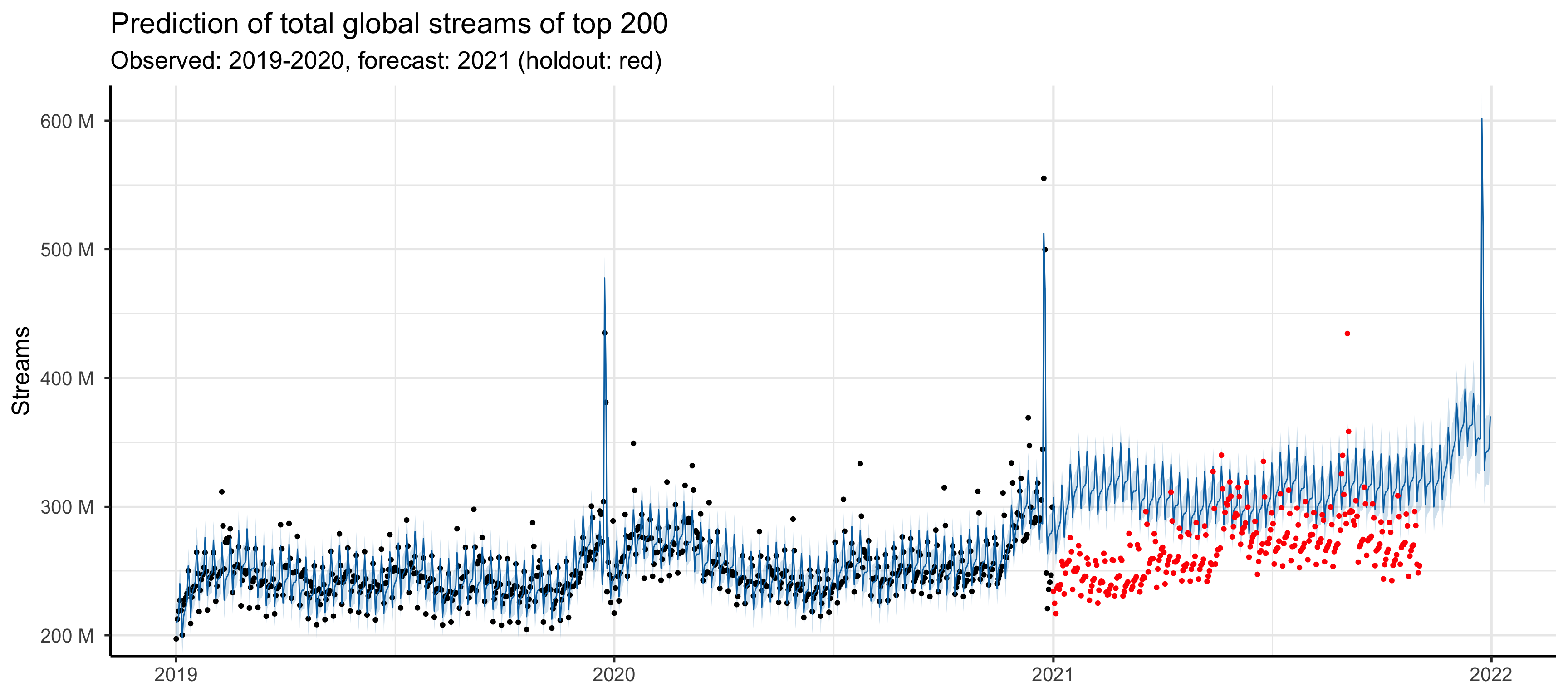
total_streams_model <- filter(total_streams, ds <= as.Date("2020-12-31"), ds >= as.Date("2019-01-01")) 
total_streams_holdout <- filter(total_streams, ds >= as.Date("2021-01-01"))
mod <- prophet(total_streams_model,
               holidays = data.frame(
                 holiday = "christmas",
                 ds = c(
                    as.Date("2019-12-25"), 
                    as.Date("2020-12-25"), 
                    as.Date("2021-12-25")),
                 lower_window = -1, upper_window = 0
               ),
               daily.seasonality = FALSE
)
future <- make_future_dataframe(mod, periods = 365)
forecast <- predict(mod, future)
plot(mod, forecast) +
  labs(
    y = "Streams",
    title = "Prediction of total global streams of top 200",
    subtitle = "Observed: 2019-2020, forecast: 2021 (holdout: red)"
  ) +
  time_series_ggstyle +
  geom_point(data = total_streams_holdout, 
  aes(x = as.POSIXct(ds), y = y), color = 'red')

What about Causality?

Causal inference and Prediction

• Variables can be predictive without a causal relationship
• Correlation does not imply causation
• Arcade revenue predicts CS doctorates (and vice versa)

• Variables can be bad predictors but have a causal relationship
• No correlation does not imply no causation
• Fuel used and speed on cruise control (uphill vs. flat)

• Variables can be predictive while not being predictive

Correlation does not even imply correlation

Andrew Gelman

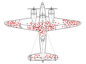
Selection bias

• For which “population” is the sample representative?

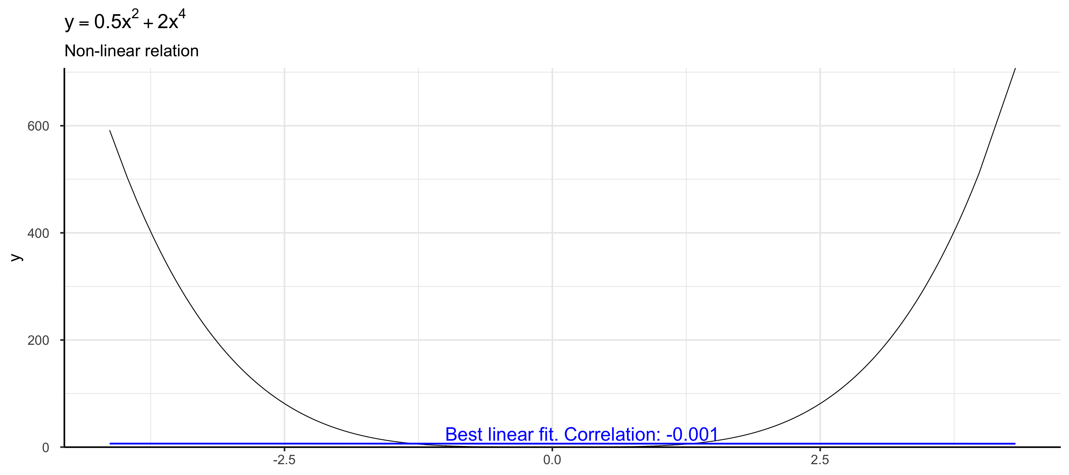
Causal but no correlation

set.seed(123)
xy <- data.frame(x = rnorm(100000))
xy$y <- 0.5 * xy$x^2 + 2 * xy$x^4
ggplot(xy, aes(x = x, y = y)) +
geom_line() +
geom_smooth(method = "lm", color = "blue") +
labs(title = expression(y == 0.5 * x^2 + 2 * x^4), subtitle = "Non-linear relation") +
annotate("text",
x = -1, y = 25,
label = paste0(
"Best linear fit. Correlation: ",
round(cor(xy$x, xy$y), 3)
), hjust = 0, color = "blue", size =8
) +
time_series_ggstyle

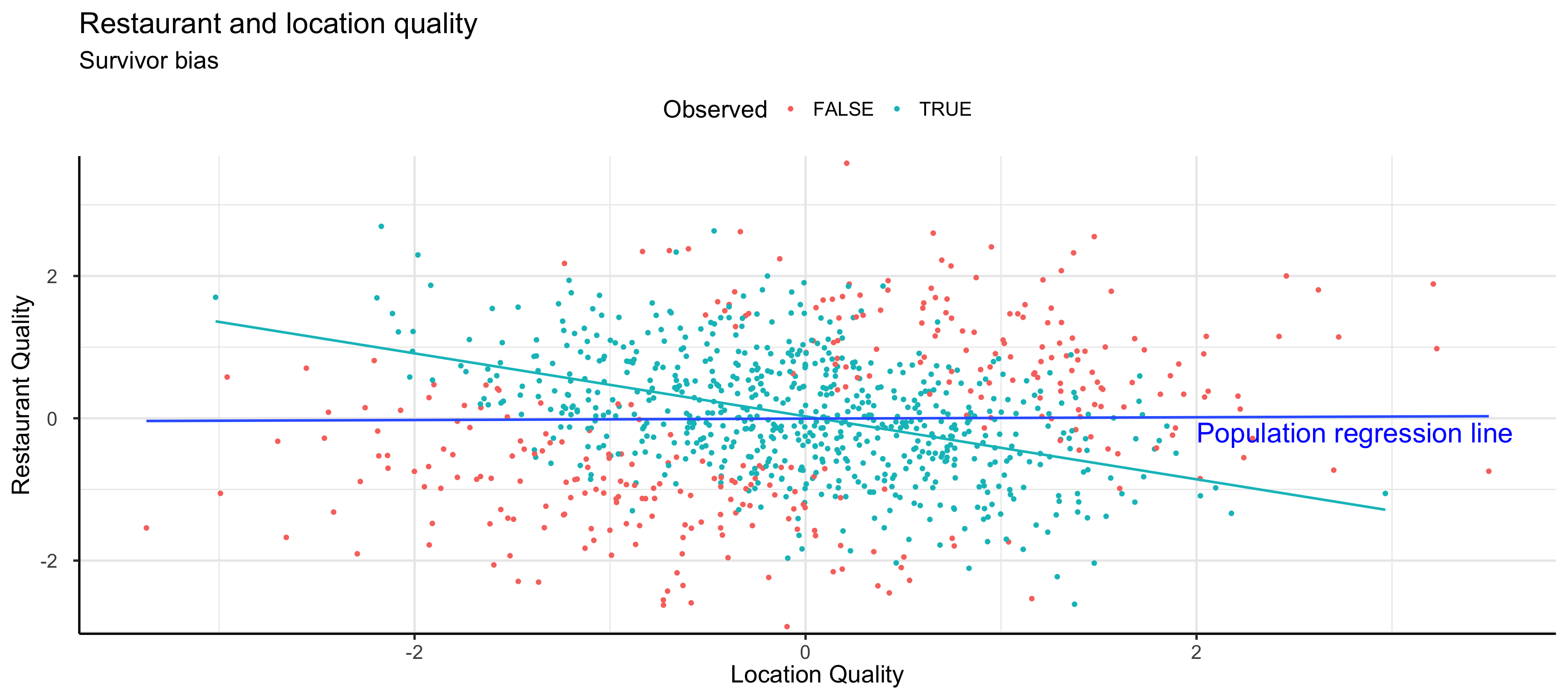
Correlation without Correlation

set.seed(42)
xy <- data.frame(x = rnorm(1000), y = rnorm(1000))
xy$obs <- abs(xy$x + xy$y) < 0.5 + runif(1000,0,2)
ggplot(xy, aes(x=x, y=y)) +
    geom_point(aes(color=obs)) +
    geom_smooth(data = xy[xy$obs,], 
    method = 'lm', se = FALSE, color = "#00BFC4") +
    geom_smooth(method = 'lm', se = FALSE) +
    time_series_ggstyle +
    labs(color = "Observed",
        title = "Restaurant and location quality", 
        subtitle="Survivor bias",
        y = "Restaurant Quality", x = "Location Quality") +
    annotate('text', 
            x = 2, y = -0.2, hjust=0,
            label = "Population regression line",
            color = "blue", size = 8 ) +
    theme(axis.title.x = element_text())

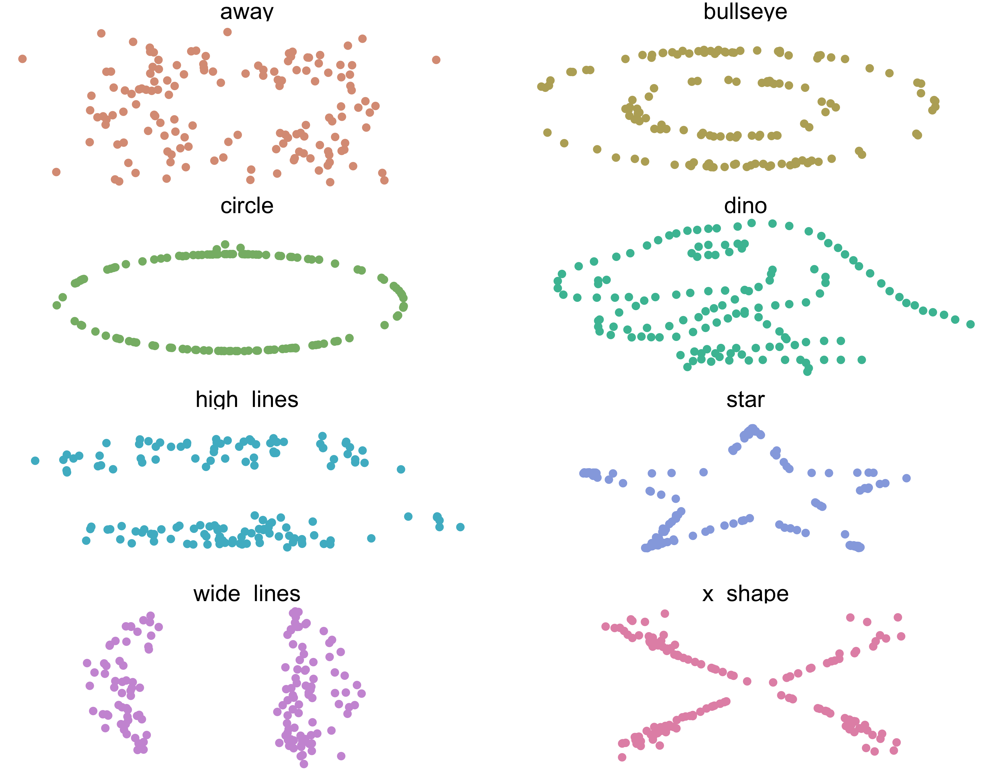
Correlation but different but still Correlation

Equivalent datasets based on estimate

library(datasauRus)
library(kableExtra)
suppressPackageStartupMessages(library(dplyr))
data <- datasaurus_dozen %>%
filter(dataset %in% c(
"away",
"bullseye",
"circle",
"dino",
"high_lines",
"wide_lines",
"x_shape",
"star"
))
data %>%
group_by(dataset) %>%
summarize(
mean_x    = round(mean(x), 2),
mean_y    = round(mean(y), 2),
std_dev_x = round(sd(x), 2),
std_dev_y = round(sd(y), 2),
corr_x_y  = round(cor(x, y), 2)
) %>%
mutate(dataset = stringr::str_replace(dataset, "_", " ")) %>%
kbl(
col.names =
c("data", "mean x", "mean y", "sd x", "sd y", "corr x,y"),
format = "html", table.attr = "style='width:100%;'"
) %>%
column_spec(1, width = "3cm")

data	mean x	mean y	sd x	sd y	corr x,y
away	54.27	47.83	16.77	26.94	-0.06
bullseye	54.27	47.83	16.77	26.94	-0.07
circle	54.27	47.84	16.76	26.93	-0.07
dino	54.26	47.83	16.77	26.94	-0.06
high lines	54.27	47.84	16.77	26.94	-0.07
star	54.27	47.84	16.77	26.93	-0.06
wide lines	54.27	47.83	16.77	26.94	-0.07
x shape	54.26	47.84	16.77	26.93	-0.07

Always visualize

library(ggplot2)
library(colorspace)
ggplot(data, aes(x = x, y = y, colour = dataset)) +
geom_point(size = 4.5) +
theme_void() +
theme(
legend.position = "none",
strip.text.x = element_text(size = 30)
) +
facet_wrap(~dataset, nrow = 4) +
scale_color_discrete_qualitative(palette = "Dynamic")

Quality of music and income

• Data: Ratings by music experts, genre, streams
• Question: Causal effect of rating on income

library(modelsummary)
library(gt)
set.seed(1)
N <- 5000
genre <- rbinom(N, 1, 0.5)
perfect_rating <- as.factor(rbinom(N, 5, 0.8 - 0.7 * genre)>4)
streams <- rexp(N, 0.01 - 0.003 * genre) |> floor()
modelsummary(
    list(lm(streams~perfect_rating),
    lm(streams~genre),
    lm(streams~perfect_rating + genre)),
    coef_rename = c("perfect_ratingTRUE" = "perfect rating"),
    stars = TRUE,
    statistic = "{p.value}",
    gof_map = NA)

	(1)	(2)	(3)
+ p
(Intercept)	122.711***	97.408***	97.314***
perfect rating	-25.112***		0.285
			0.956
genre		43.268***	43.361***

Grades and happyness

• Data: grades, self_esteem index, happyness index
• Question: Causal effect of grades on happyness

set.seed(42)
range_normalize <- function(x, min_range = 0, max_range = 100){
  x_norm <- min_range + (x - min(x)) * (max_range - min_range) / (max(x) - min(x))
}
grades <- 1 + rbinom(N, 4, 0.04)
self_esteem <- range_normalize(100 * (1/grades + rnorm(N)))
happyness <- range_normalize(5 + self_esteem + rnorm(N))
modelsummary(
    list(lm(happyness~grades),
    lm(happyness~self_esteem),
    lm(happyness~grades+self_esteem)),
    coef_rename = c("self_esteem" = "self esteem"),
    stars = TRUE,
    statistic = "{p.value}",
    gof_map = NA)

	(1)	(2)	(3)
+ p
(Intercept)	61.393***	1.510***	1.551***
grades	-5.958***		-0.029
			0.430
self esteem		0.989***	0.988***

Restaurant and location ratings

• Data: Restaurant ratings, location ratings, restaurant survival prob.
• Question: Causal effect of location rating on restaurant rating

set.seed(14)
restaurant_rating <- 25 + 10*rnorm(N)
location_rating <- 5*rnorm(N)
survival_probability <- range_normalize(0.8*restaurant_rating + 0.8 * location_rating + 10*rnorm(N), 0, 100)
modelsummary(
    list(lm(restaurant_rating~location_rating),
    lm(restaurant_rating~survival_probability),
    lm(restaurant_rating~survival_probability + location_rating)),
    coef_rename = c(
                    "location_rating" = "location rating",
                    "survival_probability" = "survival prob."
                    ),
    stars = TRUE,
    statistic = "{p.value}",
    gof_map = NA)

	(1)	(2)	(3)
+ p
(Intercept)	24.875***	3.151***	0.996*
			0.023
location rating	0.022		-0.390***
	0.440
survival prob.		0.414***	0.455***

Causal Inference: two approaches (Imbens 2020)

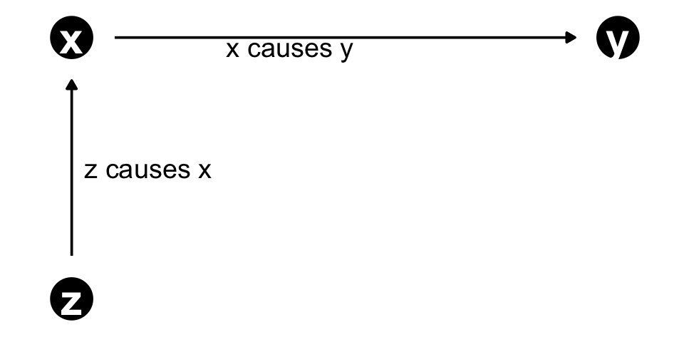
• Directed Acyclic Graphs (DAGs)
• Concerned with identification of causal relationships
• Shows direction of causality and important variables
• Graphical representation:

library(ggdag)
library(dagitty)
library(tidyverse)
dagify(y ~ x, x ~ z, exposure = "x", outcome = "y",
       coords = list(x = c(x = 1, y = 1.5, z = 1), y = c(x=1, y = 1, z=0))
) %>% 
  tidy_dagitty() %>%
  ggdag(text_size = 8, node_size = 10) +
  geom_dag_edges() +
  annotate("text", x = 1.2, y = 1, vjust=1, label= "x causes y", size=5 ) + 
  annotate("text", x = 1, y = 0.5, hjust=-0.1, label="z causes x", size = 5) +
  theme_dag()

• Potential Outcome
• Multiple Treatments / Causes
  e.g., exposure to ad
• Potential outcomes f. treatments
  e.g., Purchase given exposure / no exposure
• Multiple observations with different treatments
  e.g., A/B test
• Focus on assignment of treatment
  e.g., randomized experiment, selection on (un)observables

\[ \begin{aligned} y_i(0)& \ldots \text{outcome of individual }i\text{ without treatment} \\ y_i(1)& \ldots \text{outcome of individual }i\text{ with treatment} \\ \delta_i = y&_i(1) - y_i(0) \ldots \text{treatment effect of individual }i \end{aligned} \]

• Observed: \(y_i = D_i * y_i(1) + (1-D_i) * y_i(0)\) where \(D_i\) is the treatment indicator

Analyzing DAGs: d-separation

• Necessary to decide which variables to use in model
• “d” stands for “directional”
• Usually we are dealing with more than two variables
• Complication: causation flows only directed - association might flow against

dagify(z ~ x, y2 ~ z, a ~ x, a ~ y3, x ~ d, y1 ~ d,
       coords = list(x = c(x = 1, z = 1.5, y2 = 2, a = 1.5, y3 = 2, d = 1.5, y1 = 2), 
                     y = c(x = 1, y2 = 1, z = 1, a = 0, y3 = 0, d = 2, y1 = 2))
) %>% 
  tidy_dagitty() %>%
  ggdag(text_size = 3, node_size = 5) +
  geom_dag_edges() +
  theme_dag() +
  labs(title= "Causal Pitchfork", subtitle = "x and y2 are d-connected but x and y1/y3 are not") +
  theme(title = element_text(size = 8))

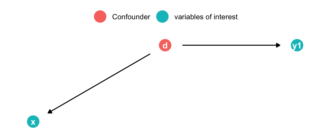
Analyzing DAGs: Fork

Good Control

med <- dagify( x ~ d, y1 ~ d,
       coords = list(x = c(x = 1, z = 1.5, y = 2, a = 1.5, b = 2, d = 1.5, y1 = 2), 
                     y = c(x = 1, y = 1, z = 1, a = 0, b = 0, d = 2, y1 = 2))
) %>% 
  tidy_dagitty() %>%
  mutate(fill = ifelse(name == "d", "Confounder", "variables of interest")) %>% 
  ggplot(aes(x = x, y = y, xend = xend, yend = yend)) + 
  geom_dag_point(size=7, aes(color = fill)) + 
  geom_dag_edges(show.legend = FALSE)+
  geom_dag_text() +
  theme_dag() +
  theme(legend.title  = element_blank(),
        legend.position = "top") 
med

• d causes both x and y1
• Arrows pointing to x are called “back-door” paths
• Eliminated by randomized experiment! Why?
• Controlling for d “blocks” the non-causal association x \(\rightarrow\) y1

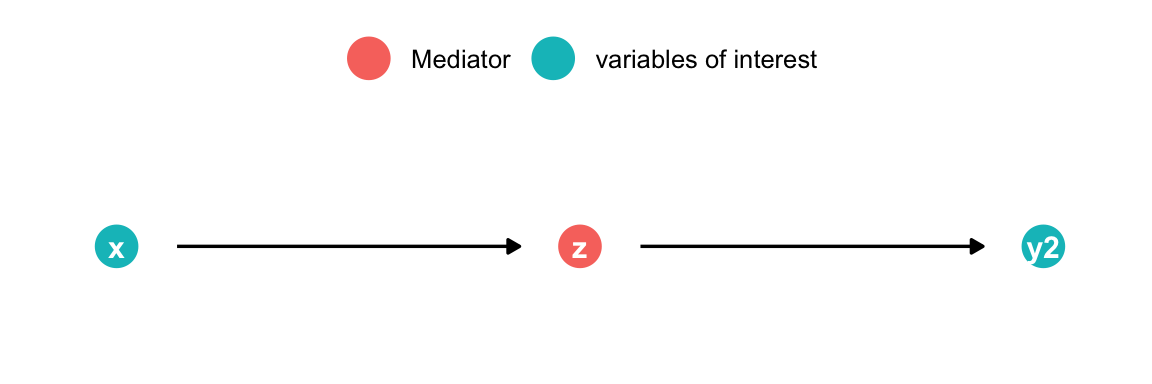
Analyzing DAGs: Pipe

Bad Control (possibly use mediation analysis)

med <- dagify(z ~ x, y2 ~ z,
       coords = list(x = c(x = 1, z = 1.5, y2 = 2), y = c(x=1, y2 = 1, z=1))
) %>% 
  tidy_dagitty() %>%
  mutate(fill = ifelse(name == "z", "Mediator", "variables of interest")) %>% 
  ggplot(aes(x = x, y = y, xend = xend, yend = yend)) + 
  geom_dag_point(size=7, aes(color = fill)) + 
  geom_dag_edges(show.legend = FALSE)+
  geom_dag_text() +
  theme_dag() +
  theme(legend.title  = element_blank(),
        legend.position = "top") 
med

• x causes y through z
• Controlling for z blocks the causal association x \(\rightarrow\) y2

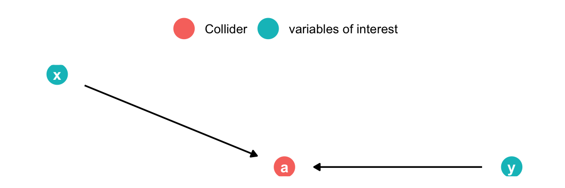
Analyzing DAGs: Collider

Bad control

dagify(a ~ x, a ~ y,
  coords = list(x = c(x = 1, y = 2, a = 1.5), y = c(x = 1, y = 0,  a = 0))
) |>
  tidy_dagitty() |>
  mutate(fill = ifelse(name == "a", "Collider", "variables of interest")) |>
  ggplot(aes(x = x, y = y, xend = xend, yend = yend)) +
  geom_dag_point(size = 7, aes(color = fill)) +
  geom_dag_edges(show.legend = FALSE) +
  geom_dag_text() +
  theme_dag() +
  theme(
    legend.title = element_blank(),
    legend.position = "top"
  )

• x & y cause a
• x & y are d-separated and uncorrelated
• By adding a to the model spurious correlation between x & y is introduced

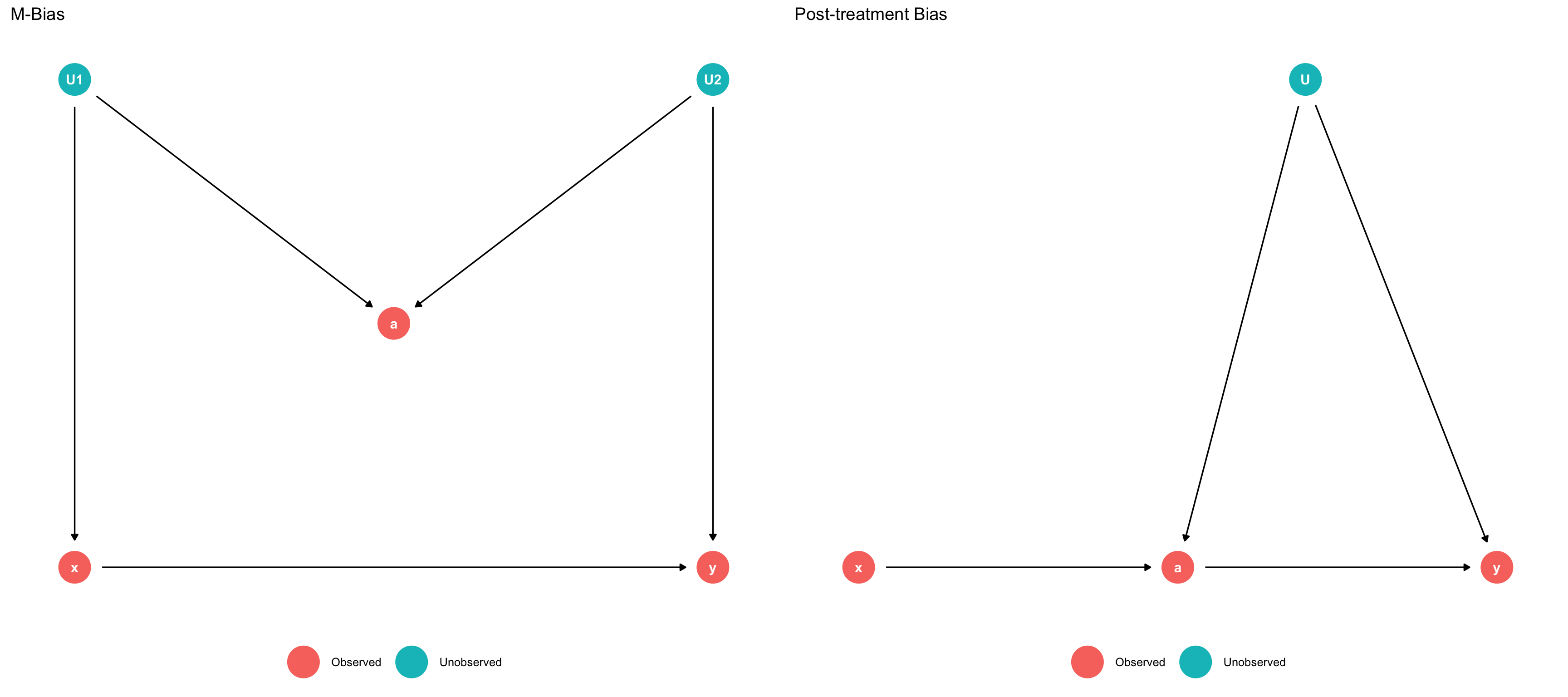
Common bad controls (Cinelli, Forney, and Pearl 2020)

library(ggpubr)
p1 <- dagify(y ~ x + U2,
       a ~ U1 + U2,
       x ~ U1,
      coords = list(x = c(x = 1, y = 2, a = 1.5, b = 1.5, U1 = 1, U2 = 2), y = c(x=1, y = 1,  a = 1.5, b = 0, U1 = 2, U2 = 2))
) %>% 
  tidy_dagitty() %>%
  mutate(fill = ifelse(name %in% c("U1", "U2"), "Unobserved", "Observed")) %>% 
  ggplot(aes(x = x, y = y, xend = xend, yend = yend)) + 
  geom_dag_point(size=12, 
                 aes(color = fill)
                 ) + 
  geom_dag_edges(show.legend = FALSE)+
  geom_dag_text() +
  theme_dag() +
  theme(legend.title  = element_blank(),
        legend.position = "bottom") +
  labs(title = "M-Bias")
p2 <- dagify(y ~ a + U,
       a ~ x + U,
      coords = list(x = c(x = 1, y = 2, a = 1.5, b = 1.5, U = 1.7, U2 = 2), y = c(x=1, y = 1,  a = 1, b = 0, U = 2, U2 = 2))
) %>% 
  tidy_dagitty() %>%
  mutate(fill = ifelse(name %in% c("U"), "Unobserved", "Observed")) %>% 
  ggplot(aes(x = x, y = y, xend = xend, yend = yend)) + 
  geom_dag_point(size=12, 
                 aes(color = fill)
                 ) + 
  geom_dag_edges(show.legend = FALSE)+
  geom_dag_text() +
  theme_dag() +
  theme(legend.title  = element_blank(),
        legend.position = "bottom") +
  labs(title = "Post-treatment Bias")
ggarrange(p1, p2)

left: M-Bias

• Do not adjust for “a” since it would open the collider path

right: Post-treatment Bias

• Do not include post treatment variable “a” since it would open the confounder path (cannot control since u is unobserved)

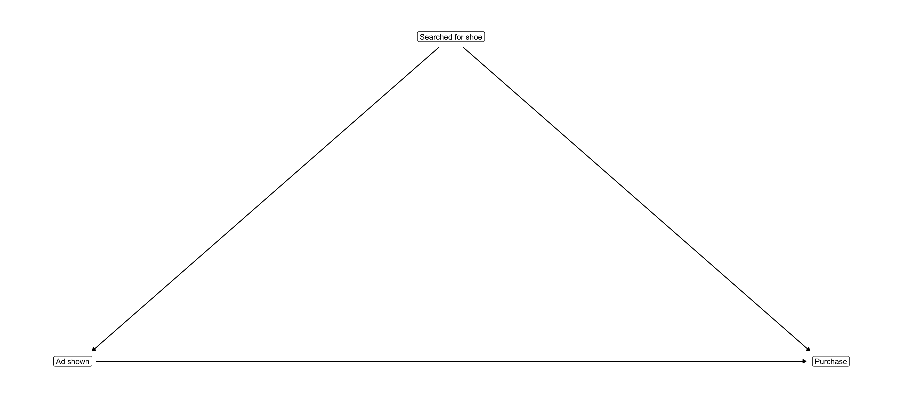
Omitted Variable Bias

library(patchwork)
suppressWarnings(library(ggdag))
library(gt)
library(dagitty)
library(ggeffects)
library(parameters)
library(marginaleffects)
confounder <- dagify(x ~ d, y ~ d, y ~ x,
  coords = list(
    x = c(x = 1, y = 2, d = 1.5),
    y = c(x = 1, y = 1, d = 2)
  )
) |>
  tidy_dagitty() |>
  mutate(
    fill = ifelse(name == "d", "Confounder", "variables of interest"),
    labs = case_when(
      name == "d" ~ "Searched for shoe",
      name == "x" ~ "Ad shown",
      name == "y" ~ "Purchase"
    )
  ) |>
  ggplot(aes(x = x, y = y, xend = xend, yend = yend)) +
  geom_dag_edges(show.legend = FALSE) +
  geom_dag_label(aes(label = labs), hjust = c(0.5, 0.7, 0.25)) +
  theme_dag() +
  theme(
    legend.title = element_blank(),
    legend.position = "top"
  )
confounder

Omitted Variable Bias

suppressPackageStartupMessages(library(stargazer))
set.seed(11)
n <- 1000
d <- 100 * rnorm(n)
x <- -4 + 0.5 * d + 10 * rnorm(n)
y <- 25 + 10 * d + 10 * rnorm(n)
stargazer(
  lm(y ~ d + x),
  lm(y ~ x), ## gamma
  lm(y ~ d), ## beta
  lm(d ~ x), ## theta
  type = 'html', keep.stat = c('adj.rsq'), single.row=TRUE)

	Dependent variable:
	y			d
	(1)	(2)	(3)	(4)
d	9.993*** (0.016)		10.005*** (0.003)
x	0.025 (0.031)	19.315*** (0.123)		1.930*** (0.012)
Constant	25.501*** (0.337)	103.471*** (6.214)	25.400*** (0.312)	7.803*** (0.621)
Adjusted R2	1.000	0.961	1.000	0.961
Note:	p<0.1; p<0.05; p<0.01

Mediation Analysis

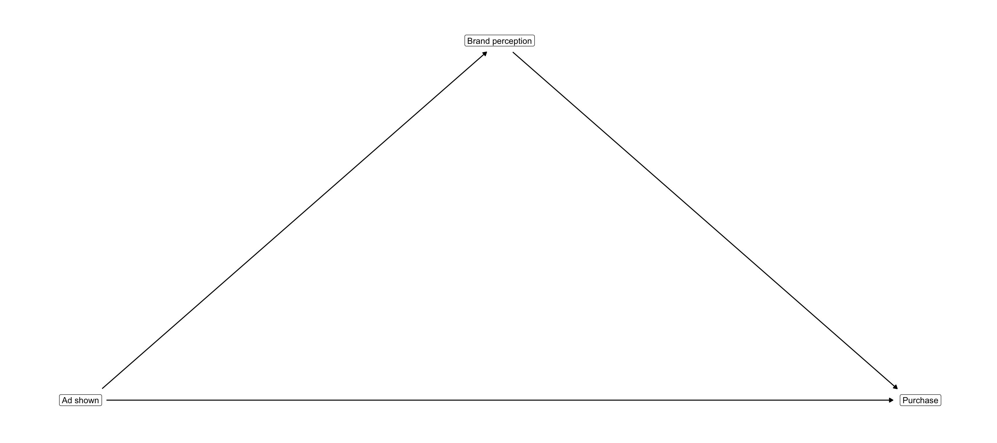
mediator <- dagify(d ~ x, y ~ d, y ~ x,
  coords = list(
    x = c(x = 1, y = 2, d = 1.5),
    y = c(x = 1, y = 1, d = 2)
  )
) |>
  tidy_dagitty() |>
  mutate(
    fill = ifelse(name == "d", "Mediator", "variables of interest"),
    labs = case_when(
      name == "d" ~ "Brand perception",
      name == "x" ~ "Ad shown",
      name == "y" ~ "Purchase"
    )
  ) |>
  ggplot(aes(x = x, y = y, xend = xend, yend = yend)) +
  geom_dag_edges(show.legend = FALSE) +
  geom_dag_label(aes(label = labs), hjust = c(0.5, 0.7, 0.25)) +
  theme_dag() +
  theme(
    legend.title = element_blank(),
    legend.position = "top"
  )
mediator

Mediation

set.seed(11)
X <- 100 * rnorm(n)
M <- 10 + 0.5 * X + 5 * rnorm(n)
Y <- -25 + 0.2 * X + 3 * M + 10 * rnorm(n)
X_on_M <- lm(M ~ X)
avg_direct_effect <- lm(Y ~ X + M)
total_effect <- lm(Y ~ X)
stargazer(
  X_on_M, 
  avg_direct_effect, 
  total_effect, 
  type = 'html', keep.stat = c('adj.rsq'), single.row=TRUE)

	Dependent variable:
	M	Y
	(1)	(2)	(3)
X	0.499*** (0.002)	0.180*** (0.031)	1.702*** (0.006)
M		3.050*** (0.063)
Constant	9.988*** (0.157)	-25.101*** (0.700)	5.364*** (0.572)
Adjusted R2	0.990	0.997	0.989
Note:	p<0.1; p<0.05; p<0.01

Moderation

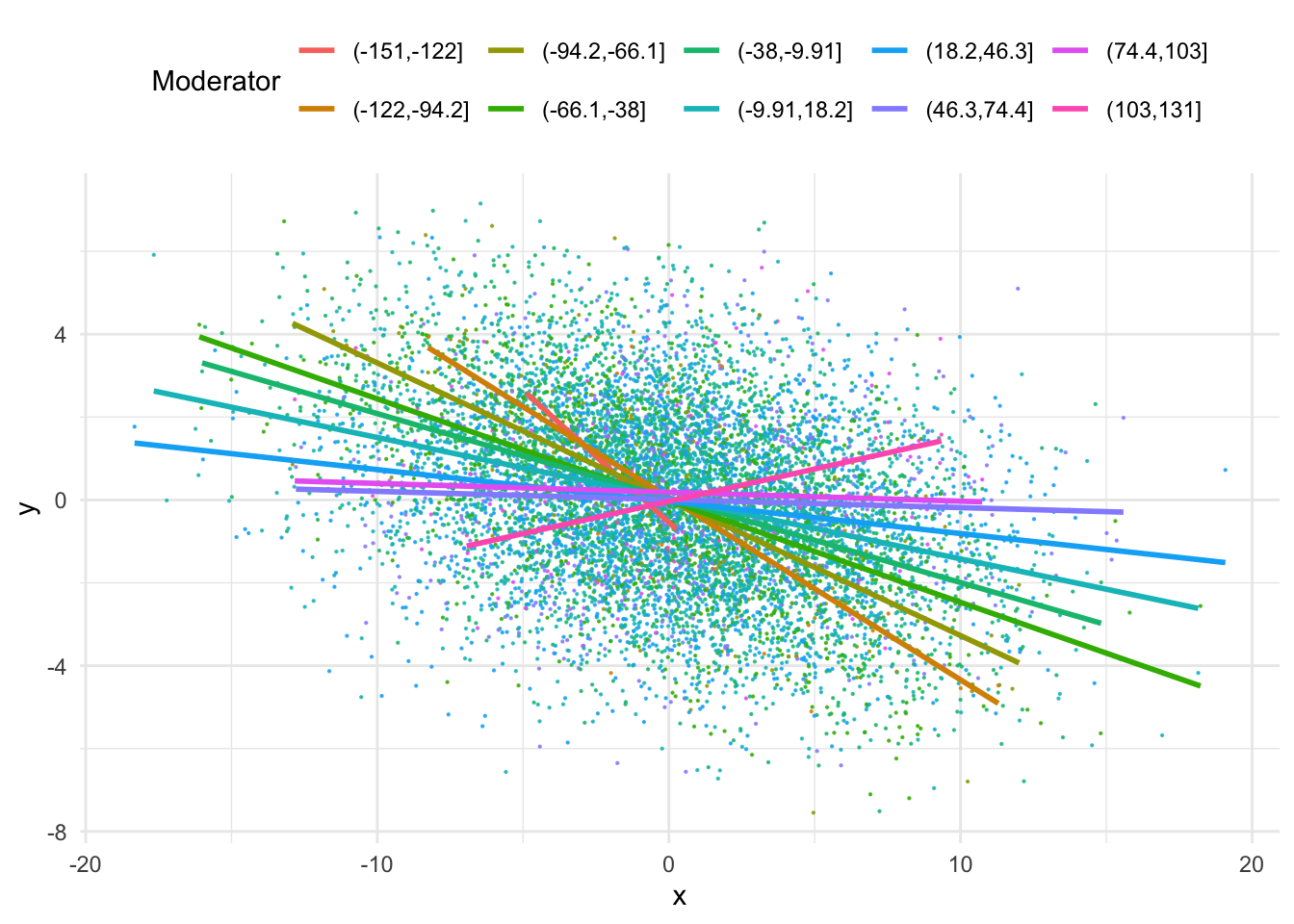
Moderation

set.seed(1)
X_mod <- rnorm(10000, 0, 5)
Moderator <- rnorm(10000, 0, 35) 
Y_mod <- -0.15 * X_mod + 0.002 * X_mod * Moderator + rnorm(10000, sd = 2)

moderation_df <- data.frame(y = Y_mod, x = X_mod - mean(X_mod), w = Moderator - mean(Moderator))
ggplot(moderation_df, aes(x = x, y = y, color = cut(w, 10))) + 
  geom_point(size = 0.1, alpha = 0.8) +
  geom_smooth(method = "lm", se = FALSE) +
  theme_minimal() +
  guides(color = guide_legend(title = "Moderator", nrow = 2)) +
  theme(legend.position = "top")

Moderation

moderated_ols <- lm(y ~ x*w, data = moderation_df)
pred_resp <- predict_response(moderated_ols, c("x", "w"))
plot(johnson_neyman(pred_resp)) 

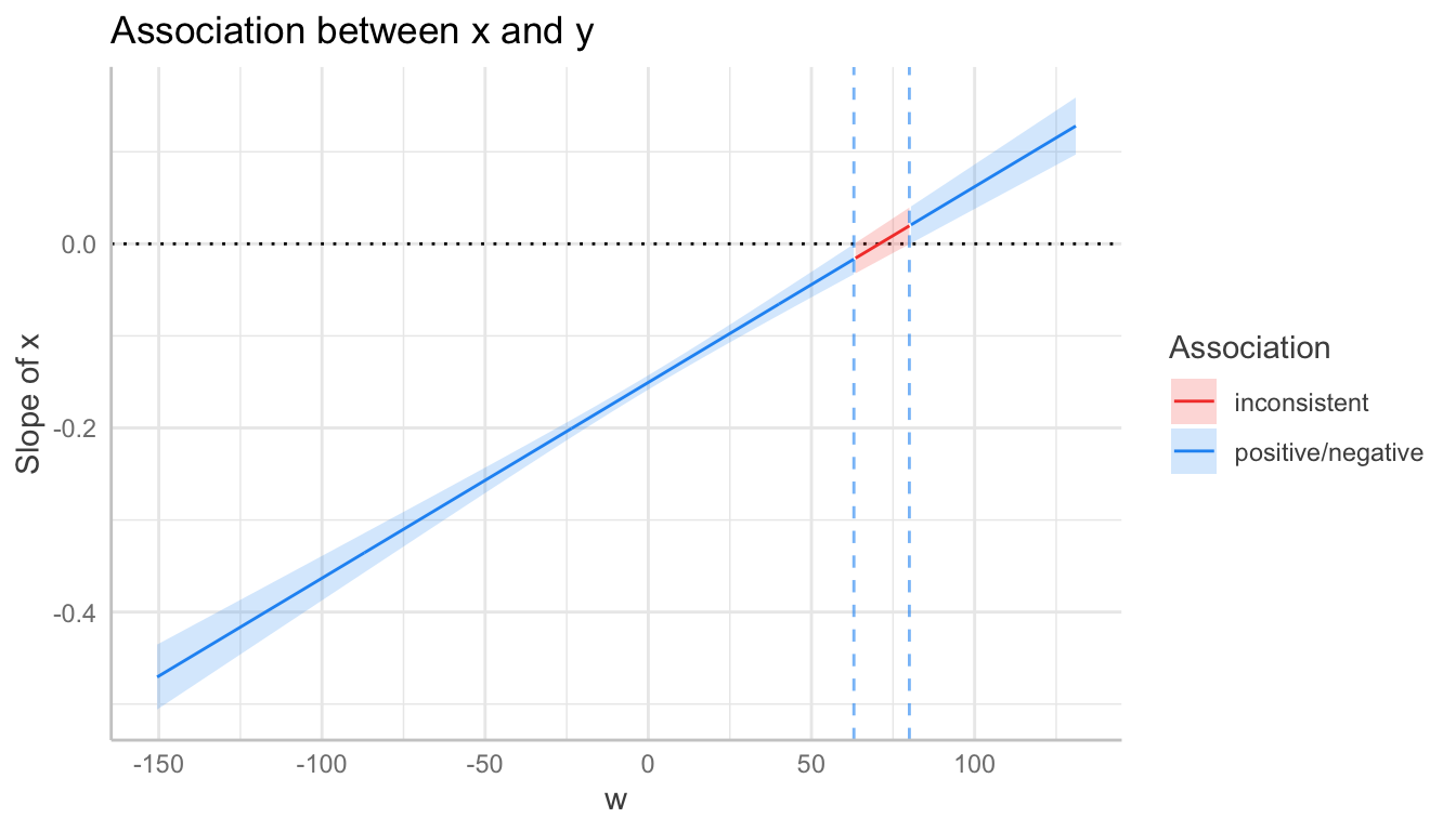
The association between `x` and `y` is negative for values of `w` lower than 63 and positive for values higher than 80. Inside the interval of [63.00,
  80.00], there were no clear associations.

Exercise

Prepare a short presentation of a (potential) DAG for your thesis

Project Topics

• Predicting sales on Amazon using linguistic features of reviews (Rocklage, Rucker, and Nordgren 2021; Filippas, Horton, and Golden 2022)
• The impact of short form video on music consumption. Cannibalisation or Promotion? - Using natural experiments to show the impact of TikTok (Callaway and Sant’Anna 2021)
• Viral online content (1): predicting virality of YouTube videos based on the sentiment of their titles (J. Berger and Milkman 2012; J. A. Berger, Moe, and Schweidel 2022)
• Viral online content (2): predicting virality of Tweets (J. Berger and Milkman 2012; J. A. Berger, Moe, and Schweidel 2022)
• Using playlists for song-success prediction (Kim et al. 2021; Pachali and Datta 2022; Boughanmi and Ansari 2021; Aguiar and Waldfogel 2021)
• Internationalization of the music industry. Analyzing international chart data (Wlömert and Papies 2019; Ordanini and Nunes 2016; Aguiar and Waldfogel 2016)
• Fraud Detection (Various topics)

References

Aguiar, Luis, and Joel Waldfogel. 2016. “Quality Predictability and the Welfare Benefits from New Products: Evidence from the Digitization of Recorded Music.” Working Paper. Working Paper Series. National Bureau of Economic Research. https://doi.org/10.3386/w22675.

———. 2021. “Platforms, Power, and Promotion: Evidence from Spotify Playlists*.” The Journal of Industrial Economics 69 (3): 653–91. https://doi.org/10.1111/joie.12263.

Berger, Jonah A., Wendy W. Moe, and David A. Schweidel. 2022. “What Holds Attention? Linguistic Drivers of Engagement.” SSRN Scholarly Paper. Rochester, NY. https://doi.org/10.2139/ssrn.4311202.

Berger, Jonah, and Katherine L. Milkman. 2012. “What Makes Online Content Viral?” Journal of Marketing Research 49 (2): 192–205. https://doi.org/10.1509/jmr.10.0353.

Boughanmi, Khaled, and Asim Ansari. 2021. “Dynamics of Musical Success: A Machine Learning Approach for Multimedia Data Fusion.” Journal of Marketing Research, April, 00222437211016495. https://doi.org/10.1177/00222437211016495.

Callaway, Brantly, and Pedro H. C. Sant’Anna. 2021. “Difference-in-Differences with Multiple Time Periods.” Journal of Econometrics, Themed issue: Treatment effect 1, 225 (2): 200–230. https://doi.org/10.1016/j.jeconom.2020.12.001.

Cinelli, Carlos, Andrew Forney, and Judea Pearl. 2020. “A Crash Course in Good and Bad Controls.” SSRN 3689437.

Filippas, Apostolos, John J. Horton, and Joseph M. Golden. 2022. “Reputation Inflation.” Marketing Science 41 (4): 733–45. https://doi.org/10.1287/mksc.2022.1350.

Imbens, Guido W. 2020. “Potential Outcome and Directed Acyclic Graph Approaches to Causality: Relevance for Empirical Practice in Economics.” Journal of Economic Literature 58 (4): 1129–79. https://doi.org/10.1257/jel.20191597.

Kim, Aekyoung, Felipe M. Affonso, Juliano Laran, and Kristina M. Durante. 2021. “Serendipity: Chance Encounters in the Marketplace Enhance Consumer Satisfaction.” Journal of Marketing 85 (4): 141–57. https://doi.org/10.1177/00222429211000344.

Ordanini, Andrea, and Joseph C. Nunes. 2016. “From Fewer Blockbusters by More Superstars to More Blockbusters by Fewer Superstars: How Technological Innovation Has Impacted Convergence on the Music Chart.” International Journal of Research in Marketing, The Entertainment Industry, 33 (2): 297–313. https://doi.org/10.1016/j.ijresmar.2015.07.006.

Pachali, Max J., and Hannes Datta. 2022. “What Drives Demand for Playlists on Spotify?” Available at SSRN.

Rocklage, Matthew D., Derek D. Rucker, and Loran F. Nordgren. 2021. “Mass-Scale Emotionality Reveals Human Behaviour and Marketplace Success.” Nature Human Behaviour 5 (10): 1323–29. https://doi.org/10.1038/s41562-021-01098-5.

Wlömert, Nils, and Dominik Papies. 2019. “International Heterogeneity in the Associations of New Business Models and Broadband Internet with Music Revenue and Piracy.” International Journal of Research in Marketing, Marketing Perspectives on Digital Business Models, 36 (3): 400–419. https://doi.org/10.1016/j.ijresmar.2019.01.007.